Showing posts with label Database. Show all posts

Wednesday, October 28, 2015

How to count the number of any day / days between two dates

Hi every one ... If we want to count the number of Saturdays and Sunday between two dates, how would we do that ? !

Dates are ( 01-Oct-2015) to (31-Oct-2015)

how to do it in SQL

SELECT TO_CHAR(dat,'DY'),COUNT(*) FROM
    (select TO_DATE('01-Oct-2015') + num dat from
    (SELECT level - 1 num
    FROM dual
    CONNECT BY level <= ABS((TO_DATE('01-Oct-2015') - TO_DATE('31-Oct-2015'))-1)))
    WHERE TO_CHAR(dat,'DY') IN ('SAT','SUN')
    GROUP BY TO_CHAR(dat,'DY')

This query helps me a lot of in my requirement, hope it helps you and fulfill your requirement as well. Also, i if you have any best solution do not forget to share as well.
Regards


AVG: What does it Mean?

AVG is an aggregate function in SQL to compute the "average" of a set of values. More precisely, it computes the mean of those values. And even more precisely, AVG computes what is known as the arithmetic mean. The underlying math is so deceptively simple, it's easy to believe one understands the result and how to apply it. But keep reading! Learning about "average" is like uncovering an iceberg. There's more to it than meets the eye.
SQL Statistic Series: You are reading part of an ongoing series covering the statistical functions available in the Oracle Database implementation of SQL.

Measure of Central Tendency

The arithmetic mean is considered a measure of central tendency. Computing such a measure is an attempt to come up with a single value through which to conveniently characterize, discuss, and compare different data sets.
Figure 1 shows the math. It's very simple: Just sum the values and divide by their quantity. The first three examples show higher values dragging the mean upward. The final example piles on some low values to drag the mean downward. What you see is characteristic of the arithmetic mean. Any value added above or below the mean will move the mean in the direction of the new value. The move may be slight, or it may be large, but it will be non-zero.
Figure 1. Examples of computing the arithmetic mean

Mean as Representative Value

An ideal use of arithmetic mean is to provide a single representative to stand in for a collection values, and you're using that representative value in some calculations. You want the math to work out as if you had looked at each value individually, but you don't want the tedium of showing each separate computation.
Example Data: Download and execute avgExamples.sql to create the example tables and data used in this article.
Pretend you're managing a combination gas station and convenience store. You're open 24 hours a day, seven days per week. It is January 2013. Your target revenue goal for the month is $500,000. Divide by 31 days in January, and you must push at least $16,129 in sales per day. The following table tracks your daily sales progress:
SELECT *
FROM daily_sales
WHERE daily_date >= DATE '2013-01-01'
  AND daily_date < DATE '2013-02-01'
ORDER BY daily_date;

DAILY_DATE          SALES_AMT
------------------ ----------
01-JAN-13               17032
02-JAN-13               15043
03-JAN-13               16783
04-JAN-13               23343
05-JAN-13               25703
06-JAN-13               19538
07-JAN-13               18001
08-JAN-13               17154
09-JAN-13               26235
10-JAN-13               14983
11-JAN-13               16010
12-JAN-13                4300
13-JAN-13                2874
Your numbers look good until the 12th, when they fall off a cliff. Freezing rain struck your area that day. Ice has played havoc on tree limbs and power lines, leaving you without power for most of two days. Gasoline has stayed in the underground tanks unpumped. Coffee pots have been cold. For two days all you've sold are potato chips and soda pop. You are worried. Your early numbers are good, but have these two days without power been enough to put you below where you need to be?
Knowing you need to average $16,129 per day for the month, you sit down at your computer and type in a query:
SELECT ROUND(AVG(sales_amt))
FROM daily_sales
WHERE daily_date >= DATE '2013-01-01'
  AND daily_date < DATE '2013-02-01';

ROUND(AVG(SALES_AMT))
---------------------
16692
Whew! This is good news. Even with those two very bad days, you're still trending above your $16,129 target. Your hard work at exceeding plan is paying off by providing you a buffer in these difficult circumstances.
Looking for even more reassurance, you query your prior two months sales:
SELECT EXTRACT (MONTH FROM daily_date) AS "Month", 
       ROUND(AVG(sales_amt)) AS "Avg Sales"
FROM daily_sales
WHERE daily_date >= DATE '2012-11-01'
  AND daily_date < DATE '2013-01-01'
GROUP BY EXTRACT (MONTH FROM daily_date)
ORDER BY EXTRACT (MONTH FROM daily_date);

     Month Avg Sales
---------- ----------
        11      18817
        12      18803
These numbers are great news. You're current mean daily sales is just barely above the line at $16,692, but your track record from the prior two months indicates significant upside potential.
For one last bit of reassurance, you decide query a running average for the month of December. You want to see how the mean daily sales changed as the month progressed. Figure 2 illustrates. Notice how each day's mean sales amount takes into account the sales history from all the prior days.
Figure 2. The concept of a running average
SQL window functions make running (and moving too) averages fairly easy. Following is a query making use ofAVG...OVER to compute the running mean daily sales for December 2012. See my article You've Got Framing! if you're unfamiliar with the OVER clause and want more detail on how it works in this scenario.
SELECT daily_date, 
       sales_amt, 
       ROUND(AVG(sales_amt) OVER (ORDER BY daily_date)) AS "Running Avg"
FROM daily_sales
WHERE daily_date >= DATE '2012-12-01'
  and daily_date < DATE '2013-01-01'
ORDER BY daily_date;

DAILY_DATE          SALES_AMT Running Avg
------------------ ---------- -----------
01-DEC-12               14530       14530
02-DEC-12               14230       14380
03-DEC-12               15830       14863
...
22-DEC-12               19235       17610
23-DEC-12               20133       17720
24-DEC-12               22839       17933
25-DEC-12               21833       18089
26-DEC-12               20593       18185
27-DEC-12               20001       18252
28-DEC-12               19848       18309
29-DEC-12               23134       18476
30-DEC-12               22783       18619
31-DEC-12               24323       18803
These results are excellent news! They show a clear and sharp movement upwards in the running average toward the end of the month. Querying for November sales, you see the very same pattern in that month. There's every reason to believe you can repeat the pattern for January. You confidently report to your regional manager that the power loss is a minor blip and nothing to be concerned about. Your daily mean sales remain above the mark; you are on track to end the month ahead of plan.
Note: Means can be useful in communicating the big picture swiftly. Recite a list of daily sales numbers and a busy manager's eyes will glaze over. Give him a single number instead, such as the mean daily sales so far in the month, and you've conveyed the big picture without burying the manager in the details.

Nulls and their Effect

SQL's AVG function ignores nulls. This is by design, and it's a good decision. If you must, you can apply a function such as COALESCE to coerce a null to some other value such as zero. Here's a trivial example to illustrate:
SELECT AVG(sales_amt) AS "Normal",
       AVG(COALESCE(sales_amt, 0)) AS "Coerced"
FROM null_demo;

    Normal    Coerced
---------- ----------
         3        1.2
And here is the underlying data:
SET NULL "NULL"
SELECT * FROM null_demo;

DAILY_DATE          SALES_AMT
------------------ ----------
01-FEB-13                   2
02-FEB-13                   4
03-FEB-13                NULL
04-FEB-13                NULL
05-FEB-13                NULL
The normal invocation of AVG takes only the non-null values 2 and 4 into account. It returns the mean as (2 + 4) / 2 = 3. The second implementation treats nulls as if they were zeros. The rather odd effect is to return a mean that does not fall between the values in the table. That mean has no meaning either. What possible business meaning can the value 1.2 convey in this scenario? None at all. Think about the following two statements:
  • Average sales are $3.00 dollars per day, but we are missing data for three of the five days.
  • Average sales are $1.20 dollars per day, and I'm going to leave you with the impression that no data is missing.
Which of these would help you make a better business decision? Would you rather hear the truth? Or bury your head in the proverbial sand?

Weighted Means

Sometimes it's not enough to simply take the average of a single column. Picture yourself a fleet manager responsible for a small fleet of delivery trucks. You're responsible for managing fuel costs to an average of $3.50 or less per gallon for the month. Fail, and you lose your bonus pay. Wanting to get a quick sense of how things are going, you execute the following query:
SELECT ROUND(AVG(PRICE),2) AS "Avg Per Gal"
FROM fleet_fuel
WHERE buy_date >= DATE '2013-01-01'
  AND buy_date < DATE '2013-02-01';

Avg Per Gal
-----------
       3.46
This result looks great. Doesn't it? You've applied the AVG function. You've gotten a result. You're well under the mark. You feel your bonus is secure. Except you're wrong.
You've forgotten to factor in the number of gallons purchased at each price. Each per-gallon purchase price needs to be weighted by the number of gallons purchased at that price. The AVG function doesn't help here. You can apply SUM instead, and do the weighting math yourself. Here's how:
  1. Begin with gallons * price to weight each price by the number of gallons sold.
  2. Apply the SUM function, as in SUM(gallons * price) to give a total off all you've spent on fuel so far during the month.
  3. Divide by the number of gallons to get the mean price per gallon.
Figure 3 illustrates this logic and why it works. Callout #1 shows the data for two fuel purchases. Callout #2 shows a naive and incorrect approach to computing the mean. You do a get mean of two values, but that mean does not mean what it should mean. Callout #3 highlights the correct approach. Multiplying each price by the number of gallons purchased at that price gives the effect of having a record for each individual gallon purchased. The resulting mean is then truly the mean price per gallon.
Figure 3. Weighting the mean
Fortunately, the needed SQL expression is far easier to write than Figure 3 was to draw. Here's a query implementing the logic from Figure 3 for a weighted mean:
SELECT ROUND(SUM(gallons * price)/SUM(gallons),2) AS "Avg Per Gal"
FROM fleet_fuel
WHERE buy_date >= DATE '2013-01-01'
  AND buy_date < DATE '2013-02-01';

Avg Per Gal
-----------
       3.52
This result's more worrisome, isn't it? Your target is $3.50 per gallon. Your current, weighted mean is $3.52 per gallon. That bonus isn't so secure after all. Fortunately, you have time left in the month to act. Good thing you knew about weighted means. You may be able to salvage that bonus yet.

When Median and Mode are Better

Say that you have a friend planning a visit to Michigan's Upper Peninsula. Your friend plans to drive across region, and asks you for some intelligence on fuel prices. Here is a situation in which the goal is not really to make the math work out accounting-style as in the examples so far. Instead, you're trying to distill a complex picture into just a few numbers that you and your friend can get a grip on. The arithmetic mean might not be your best choice here.
It may in fact be reasonable to provide the mean per-gallon fuel price. After all, gasoline is a competitive market and prices tend to cluster tightly around a center. There aren't likely to be many outliers. You could tell your friend:
"The mean fuel price in the region is $3.55 per gallon."
However, an even more meaningful statement is:
"Half the gas stations charge less than $3.50 per gallon, and half charge more."
Here you are giving what is known as the median: $3.50 per gallon in this case. This is useful information, and I plan a follow-up article soon on how to compute the median and apply it. Your friend can reasonably decide to treat $3.50 as the maximum he'll pay per gallon. Knowing that half the fuel stations charge less, and presuming a reasonably even geographic distribution, your friend should be able to make the trip and hold out for the less-expensive gas stations.
But wait! There's more. Perhaps you can provide the mode as well, also a planned future topic. The mode refers to the most commonly observed value. You investigate and find the fuel prices in your region to bebimodal. That means two prices are tied for being most commonly observed. The two prices are $3.46 and 3.52. Now you can paint a more detailed picture for your friend, and with just a very few numbers:
"Half the gas stations charge less than $3.50 per gallon, and half charge more."
"The two most common prices are $3.46 per gallon, and $3.52 per gallon."
With this information, your friend might decide to hold out for $3.46 per gallon or less. Again, that's presuming a not-too-uneven geographic distribution. (There is only so much you can convey, after all, with just three numbers).
Choosing the correct statistic isn't just about the data you're working with. You can't look at a data set and say arbitrarily that the median applies, or that the mean is a better choice. Choose your statistics based upon the intelligence you're trying to derive, the decisions you're hoping to make, the picture you want to paint.
Note: Median is in many cases more useful or desirable than the arithmetic mean. Yet SQL has a history of poor support for computing the median. (Oracle Database does currently support a MEDIANfunction). You'll find plenty of convoluted techniques in older books on SQL for computing the median, some that work well and others that work mostly – except for some corner cases. It's always been trivial to compute the mean though, and sometimes the mean has been chosen only for that reason. It's the "when all you have is a hammer" effect.

Circular Data

Watch out for circular number systems when computing the mean, or any other measure of central tendency. Look at Figure 4 showing several times clustered around midnight. A naive approach to computing the mean would put it at 12:02:15, twelve hours opposite where it ought to be. In this particular example, the mean as a measure of central tendency is correctly placed at 00:02:15, two minutes and 15 seconds past midnight.
Figure 4. Mean in a circular number system

Wall-clock time and compass direction are two examples of circular systems in which care is needed when computing the mean. Various methods exist. The United States Environmental Protection Agency employs the so-called Yamartino method developed in 1984 by Robert J. Yamartino in their studies involving wind direction. That's just the tip of the iceberg. At least one book, Statistical analysis of Circular Data by N. I. Fisher, has been written on the topic.

Non-Additive Data

The arithmetic mean is based around addition. Remember the daily sales example early in this article? Each day of the month you sell a certain amount, and you add those amounts together for a monthly total. For example:
14530 + 14230 + 15830 ... 23134 + 22783 + 24323
Two other common patterns you'll encounter involve rates and products. It's useful to know how to spot them so that you don't apply AVG when it shouldn't be applied.
Rates often involve the word "per", as in "miles per gallon" and "kilometers per hour". Imagine if I made the same 60 km trip twice in the same day. First I drove it at 60 kph. Then I returned home at a slower, 40 kph. Here's how that looks:
60km at 60kph + 60km at 40kph
This is not the simple, additive pattern to which arithmetic mean applies. The correct mean speed is not 50 kph like you might expect. It's actually 48 kph, because you spend more time (more hours) driving the slower trip. Another type of mean, the harmonic mean, will give the correct answer and should generally be applied to situations like this involving rates. The math behind the harmonic mean, and especially why that math works, is really interesting and I plan a future article on the topic.
The other commonly encountered pattern involves products – values multiplied together instead of being added. Remember during the runup to the year 2000 how all of us in the computing field would get big raises each year as the industry frantically worked to save the world from six-digit date meltdown? Those were good times. Imagine three yearly raises in pay of 10%, 20%, and 30%. Let your starting salary be N, and here's what you have:
 N * 1.10 * 1.20 * 1.30
Once again, this is not an additive sequence. Rather, it's a series of products. The mean pay raise is not 20%. The geometric mean applies here, and the mean increase in pay works out to 19.72% per year. You can prove that by working through some math:
N * 1.10 * 1.20 * 1.30 = N * 1.1972 * 1.1972 * 1.1972
1.10 * 1.20 * 1.30 = 1.7160, 
and 1.1972 * 1.1972 * 1.1972 = 1.7159,
and finally...N * 1.7160 ≈ N * 1.7159
Rounding accounts for the difference of 0.0001 in the result. Geometric mean is also a topic I plan for a future article.

The Sum of it All

Choose your average carefully depending upon what it is you're trying to convey. Arithmetic mean is ideal when you need the math to work out accounting-style, as in the daily sales and fuel cost examples. Watch for non-additive cases that might require other types of mean, such as the harmonic and geometric.
Arithmetic mean is prone to what is termed skew. A small number of outlying values can give a false impression of central tendency. Figure 1 hints at how this may be so. A future article on standard deviation will delve into this topic more closely.
The potential for skew is one reason the median is often favored over the mean. This is why the U.S. Census Bureau tracks and reports a median  annual household income rather than a mean income. Median is often more appropriate than the mean in cases where you are working to promote understanding  by painting a picture of the current state of things.
Finally, it isn't possible to look at a data set and declare authoritatively that just one statistic applies, or that only one type of average should be used. It may be perfectly reasonable to look at multiple statistics together, such as mean and mode in the example of an automobile trip across the Upper Peninsula. The bottom line is to choose the statistic that best conveys the message, and that best helps you manage to your desired result.

Dates in Range

Posing the Question

Arturo was after a solution encompassing more than a single month. Following is the question he put to me:
"What if you had two different ranges?
   beg_date        end_date
   01-Jan-2013     15-Jan-2013
   15-Mar-2013     02-Apr-2013
How do you generate individual rows for each day between 01/01 to 01/15, and between 03/15 to 04/02?"
An excellent question! Arturo's question forces me to gereralize the solution from my previous article that is specific to days in a single month, and make it work to cover any date range, even one spanning many months.

Getting Started

Following is my starting point, the solution from my prior article. It's a query that returns one row for each day in the current month.
SELECT LEVEL, LAST_DAY(SYSDATE)-LEVEL+1
FROM dual
WHERE ROWNUM <= EXTRACT(DAY FROM LAST_DAY(SYSDATE))
CONNECT BY LEVEL=ROWNUM;
The query makes creative use of LEVEL and CONNECT BY to form a row-generator giving incremental values beginning with 1. Following are some aspects to consider:
  • The LEVEL column counts upward toward the number of days in the month.
  • The starting date is implicitly the first of the month.
  • The EXTRACT expression generates a value marking the end of the range.
The solution logic is based around integers returned by LEVEL and EXTRACT that represent day numbers. That logic limits the solution to generating rows for only a single month.

Generalizing the Solution

My first need is to generalize the query by making it possible to specify any two dates to denote the range of interest. Before doing that, I want to get rid of ROWNUM from the WHERE clause and use LEVEL instead. It may be lack of coffee, but my use of ROWNUM is making it harder for me to think clearly about the query and how it works. The fix is a trivial, one-word change to the WHERE clause:
SELECT LEVEL, LAST_DAY(SYSDATE)-LEVEL+1
FROM dual
WHERE LEVEL <= EXTRACT(DAY FROM LAST_DAY(SYSDATE))
CONNECT BY LEVEL=ROWNUM;
Now I can get on with solving the problem at hand. I want to specify beginning and ending dates explicitly. There are two date ranges, so I'll create and initialize four bind variables in SQL*Plus:
VARIABLE beg1_date CHAR(11);
VARIABLE end1_date CHAR(11);
VARIABLE beg2_date CHAR(11);
VARIABLE end2_date CHAR(11);

EXECUTE :beg1_date := '1-Jan-2013'; 
EXECUTE :end1_date := '15-Jan-2013';
EXECUTE :beg2_date := '15-Mar-2013';
EXECUTE :end2_date := '2-Apr-2013';
My solution query shown earlier generates dates in reverse order, beginning from the end of the month as given by LAST_DAY(SYSDATE). It's an easy modification to reference end2_date as the end of the range. Just specify TO_DATE(:end2_date) instead. For example:
From: SELECT LEVEL, LAST_DAY(SYSDATE)-LEVEL+1
To: SELECT LEVEL, TO_DATE(:end2_date)-LEVEL+1
I'll simplify the WHERE clause to restrict output to ten rows. Let's see how things go:
SELECT LEVEL, TO_DATE(:end2_date)-LEVEL+1
FROM dual
WHERE LEVEL <= 10
CONNECT BY LEVEL=ROWNUM;

     LEVEL TO_DATE(:END2_DATE
---------- ------------------
         1 02-APR-13
         2 01-APR-13
         3 31-MAR-13
         4 30-MAR-13
         5 29-MAR-13
         6 28-MAR-13
         7 27-MAR-13
         8 26-MAR-13
         9 25-MAR-13
        10 24-MAR-13
These results are promising. Next I can modify the WHERE clause to terminate execution at the beginning of the range. I'll specify beg1_date, because I want the query to generate a wide enough range of dates to encompass both the desired, smaller ranges. Here's the query and its results:
SELECT LEVEL, TO_DATE(:end2_date)-LEVEL+1
FROM dual
WHERE TO_DATE(:beg1_date) <= TO_DATE(:end2_date)-LEVEL+1
CONNECT BY LEVEL=ROWNUM;

     LEVEL TO_DATE(:END2_DATE
---------- ------------------
         1 02-APR-13
         2 01-APR-13
         3 31-MAR-13
...
        90 03-JAN-13
        91 02-JAN-13
        92 01-JAN-13
The query is now generating an extended range of dates covering both the smaller ranges that I'm after.

Punching a Hole

All that's left is to "punch a hole" in the results by getting of the unwanted rows. Here is my first attempt, which is to add two predicates to the WHERE clause:
SELECT LEVEL, TO_DATE(:end2_date)-LEVEL+1
FROM dual
WHERE TO_DATE(:beg1_date) <= TO_DATE(:end2_date)-LEVEL+1
  AND NOT (
        TO_DATE(:end2_date)-LEVEL+1 > TO_DATE(:end1_date)
    AND TO_DATE(:end2_date)-LEVEL+1 < TO_DATE(:beg2_date)
    )
CONNECT BY LEVEL=ROWNUM;

     LEVEL TO_DATE(:END2_DATE
---------- ------------------
         1 02-APR-13
         2 01-APR-13
         3 31-MAR-13
...
        17 17-MAR-13
        18 16-MAR-13
        19 15-MAR-13
Bummer! The CONNECT BY logic falls into the hole and terminates. Results are good until the desired gap is encountered. Then query execution ends.

Playing the Crazy Card

What's needed is a second WHERE clause. The HAVING clause can serve that purpose if you group by all the columns. The result is a fun query that you should probably not ever use in a production setting:
SELECT LEVEL, TO_DATE(:end2_date)-LEVEL+1
FROM dual
WHERE TO_DATE(:beg1_date) <= TO_DATE(:end2_date)-LEVEL+1
CONNECT BY LEVEL=ROWNUM
GROUP BY LEVEL, TO_DATE(:end2_date)-LEVEL+1
HAVING NOT (
        TO_DATE(:end2_date)-LEVEL+1 > TO_DATE(:end1_date)
    AND TO_DATE(:end2_date)-LEVEL+1 < TO_DATE(:beg2_date)
    )
ORDER BY LEVEL;

     LEVEL TO_DATE(:END2_DATE
---------- ------------------
         1 02-APR-13
         2 01-APR-13
         3 31-MAR-13
...
        17 17-MAR-13
        18 16-MAR-13
        19 15-MAR-13
        78 15-JAN-13
        79 14-JAN-13
        80 13-JAN-13
...
        90 03-JAN-13
        91 02-JAN-13
        92 01-JAN-13
The ORDER BY clause I've added this time is irrelevant to the logic. It merely undoes the effects of the grouping operation so the results are displayed in a comprehensible order.

Finding Some Sanity

While clever, the preceding approach is pretty awful. The grouping operation is likely to force a partial sorting of the data. It surely must be better to avoid the GROUP BY processing. To that end, take a query and subquery approach:
SELECT day_of_range FROM (
SELECT LEVEL AS range_counter, 
       TO_DATE(:end2_date)-LEVEL+1 AS day_of_range
FROM dual
WHERE TO_DATE(:beg1_date) <= TO_DATE(:end2_date)-LEVEL+1
CONNECT BY LEVEL=ROWNUM
) WHERE NOT (
        day_of_range > TO_DATE(:end1_date)
    AND day_of_range < TO_DATE(:beg2_date)
    );
The inner query generates the extended range of dates. The outer query's WHERE clause punches the desired hole in that range. The results are dates covering just the two, smaller ranges.

Pondering an Alternative

If the desired gap is large enough, then you may prefer to attack the problem as a union of two queries. Be sure to use the UNION ALL operator to avoid the overhead of unneeded elimination of duplicate rows; there won't be any. For example:
SELECT LEVEL, TO_DATE(:end2_date)-LEVEL+1
FROM dual
WHERE TO_DATE(:beg2_date) <= TO_DATE(:end2_date)-LEVEL+1
CONNECT BY LEVEL=ROWNUM
UNION ALL
SELECT LEVEL, TO_DATE(:end1_date)-LEVEL+1
FROM dual
WHERE TO_DATE(:beg1_date) <= TO_DATE(:end1_date)-LEVEL+1
CONNECT BY LEVEL=ROWNUM;
The first query in this union generates the latter range. The second query generates the earlier range.

Tuesday, March 5, 2013

PHP Database Driven Website


You can use PHP, (in conjunction with SQL and HTML), to create database driven websites.
To create a database driven website in PHP, you need a database management system (DBMS). Common database systems include MySQL, Microsoft SQL Server, and Oracle.
Your DBMS can be located either on the same computer that the website is on, or on another server. It's good practice to separate your database server from your web server, but if you've only got one machine to develop on, sharing the same machine shouldn't cause any problems (as long as it's powerful enough to run a web server and database server etc).
Anyway, once you have a database with some tables and some data, you can connect to it and query it.
MySQL is a database system commonly used with PHP websites. The following examples demonstrate how to connect and query a MySQL database.

Connecting to the Database

Before you can query your database, you need to connect to the database server, then locate the database. Once you've done this, you can send in your SQL code to do your queries.
To connect to the database server:
Code

The above code uses the mysql_connect function to connect to the database server. We provide the following parameters: Server, Username, Password. PHP needs this info so that it knows which server to connect to. In this example we are just connecting to the local machine so we use "localhost" as the server.
We have also used the PHP die and mysql_error functions to be used in the event there's an error and PHP can't connect to the server. This will display the error message which can assist us in determining the cause of the problem.
To select the database:
Code

The above code uses the mysql_select_db function to select the database from the database server. You need to do this because, your database server could contain many databases. You need to tell PHP which database to use.
Again we use the die and mysql_error functions to be used in the event of an error.

Querying the Database

You can use the mysql_query function to send a SQL query to the database:
Code

What we do here is, assign the results of a query to the $result variable. The query is acheived by passing a SQL statement to the mysql_query as a parameter. In this SQL statement, we are selecting all records from the "Individual" table.
Once again we use the die and mysql_error in case there's an error.

Displaying the Results

To display the results, you need to loop through the results of the query and display each record with each iteration of the loop:
Code

Here we use a while loop to loop through the results of the query. The while loop keeps iterating until it finishes the last result. This means we can display each result as it iterates past that result. We display the result using $echo and the PHP $row variable, indicating which columns we want to display.

The Whole Code

Combining the above code, (and adding comments), results in something like this:
Code

Database Summary


So, you've made it to the last page of this database tutorial... Well done!
You should now have a general understanding about databases and how they're used. This tutorial was intended for beginners trying to gain an understanding of databases. Databases are not like most other files and require a little bit of thought in order for you to understand the concept.
If you have your own database management system installed, you should have a better understanding of where to start and what the various options mean.

What Next?

Most of the examples in this tutorial used Microsoft Access. 
Also, you'll have noticed SQL coming up throughout this tutorial. SQL is a very powerful language, but is also very easy to learn. You can achieve a lot even by learning just a little SQL. Once you complete this tutorial, you will be able to do things such as:
  • Select only the columns you want from a query
  • Query multiple tables
  • Create databases programatically
  • Create tables programatically
  • Query multiple tables
  • Use built-in functions
  • Create an index
  • And more...

Database Driven Website


A database driven website is a website that has most of its webpage content in a database. Therefore, the website content isn't actually sitting in files on the server, it is sitting in tables and columns in a database.
A website with its content stored on the file system is often referred to as a static website, whereas a database driven website is often referred to as a dynamic.

Content Management Systems

A website with dynamic content usually has a CMS (Content Management System) to assist the content providers in updating the website.
A CMS is usually provided in the form of an administration area where content providers need to log in before they can add content. Once logged in, they can create, update and delete articles. They may be able to upload files such as Word documents, PDF files etc. They might be able to upload images too.
All of this content can be stored in the database. Some may be stored on the file system too though. For example, although documents and images can be stored in the database, there are sometimes reasons to store them on the file system. Performance is often a key reason. Database size is another.

Discussion Forums and Blogs

Discussion forums and blogs have become a popular feature for many websites. Most, if not all, forums and blogs are database driven. Users can register their details, then add content. When the user clicks the "Submit" button, their details/content is inserted into the database. Then when someone decides to view this content, it is read from the database using SQL (Structured Query Language).

Combination of Static and Dynamic

Some websites have a combination of static content and dynamic content. There could be any number of reasons for this. Often, smaller websites will be static. There's little need to configure a database just to store a handful of webpages - much easier and cheaper to keep them as files on the server. Even websites like this might contain some added functionality such as a discussion forum, or a blog. In this case, the discussion forum or blog will need its content stored in a database.

Benefits of a Database Driven Website

Database driven websites can provide much more functionality than a static site can. Extended functionality could include:
  • Enabling many (potentially non-technical) users to provide content for the website. Users can publish articles on the website without needing to FTP them to a web server.
  • Shopping cart
  • You can provide advanced search functionality that enables users to filter the results based on a given field. They can then sort those results by a field - say "Price" or "Date".
  • Customized homepage
  • You can allow your users to perform tasks such as registering for a newsletter, post questions to your forums, provide comments on a blog, update their profile, etc.
  • Integration with corporate applications such as CRM systems, HR systems etc
  • Much more

Creating a Database Driven Website

The most common tasks for database driven websites is inserting, updating, and deleting data. Some of these are the same tasks that you learned in this tutorial, however when using a database driven website, you need to use a different method to do these tasks. You need to use a programming language called SQL (Structured Query Language) to insert, update, and delete your data.
Don't worry, this is not as scary as it may sound. SQL is a very easy language to learn and, once you start using it, you will be thankful you took the time to learn it. In fact, you've already learned some basic SQL statements in previous lessons.
To create a database driven website, you need the following skills:
  • You need to be able to build a static website HTML, and preferrably CSS and JavaScript
  • You need to be able to write basic code using a server side scripting language such as PHP, ColdFusion etc
  • You need to know how to write basic SQL

Relational Database Design


Most popular database management systems are relational systems, and are usually referred to as Relational Database Management Systems (RDBMS). What this means is that their databases can contain multiple tables, some (or all) of which are related to each other.
For example, consider the following screenshot:
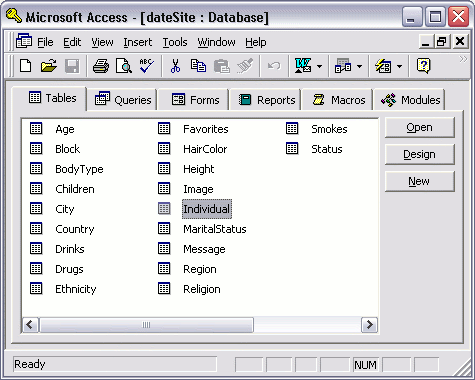
Multiple database tables
In this example, the database has 20 tables. Each table serves a specific purpose. This enables us to organize our data much better. It can also help us with theintegrity of our data.
Using the example above, the Individual table can hold data that is strictly about the individual. The City table can hold a list of all cities. If we want to know which city each individual lives, we could store a "pointer" in the Individual table to that city in the City table.
MS Access Relationships
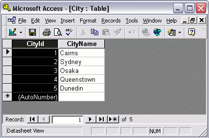
The above example demonstrates the relationship between the Individual table and the City table. The individuals in the "Individual" table live in cities that are defined in the "City" table. Therefore, we can cross-reference each "Individual" record with a "City" record.

How Does This Work?

Firstly, in the City table, each record has a unique identifier. A unique identifier is a value that is unique to each record. This identifier can be as simple as an incrementing number. So, in our City table, the first record has a number of 1, the second record has a number of 2, and so on.
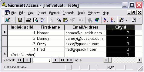
Secondly, when entering each individual into the Individual table, instead of writing out the full city name in that table, we only need to add the city's unique identifier. In this case, the unique identifier is a number, so we enter this number into the "CityId" column of the "Individual" table.
The following screenshots demonstrate this:
Relational Databases Example 2

Relational Databases Example 3
So, by looking at both tables, we can determine that Homer lives in Sydney, Barney lives in Cairns, and both Ozzy and Fred live in Osaka. At this stage, nobody in our database lives in Queenstown or Dunedin.

Primary Keys and Foreign Keys

Primary keys and foreign keys are terms that you will become very familiar with when designing databases. These terms describe what role each of the columns play in their relationship with each other.
The column that contains the unique identifier is referred to as the Primary Key. So, in our City table, the primary key is the CityId column.
foreign key is the column in the other table that points to the primary key. Therefore, the CityId column in the Individual table is a foreign key to the CityId column in the City table.

Querying a Database


Queries are one of the things that make databases so powerful. A "query" refers to the action of retrieving data from your database. Usually, you will be selective with how much data you want returned. If you have a lot of data in your database, you probably don't want to see everything. More likely, you'll only want to see data that fits a certain criteria.
For example, you might only want to see how many individuals in your database live in a given city. Or you might only want to see which individuals have registered with your database within a given time period.
As with many other tasks, you can query a database either programatically or via a user interface.

Option 1: Programatically

The way to retrieve data from your database with SQL is to use the "SELECT" statement.
Using the SELECT statement, you can retrieve all records...
Code

...or just some of the records:
Code

The 2nd query only returns records where the value in the "FirstName" column equals "Homer". Therefore, if only one individual in our database had the name "Homer", that person's record would be shown.
Something like this:
Results of a database query
SQL is a powerful language and the above statement is very simple. You can use SQL to choose which columns you want to display, you could add further criteria, and you can even query multiple tables at the same time. If you're interested in learning more about SQL, be sure to check out our SQL tutorial after you've finished this one!

Option 2: User Interface

You might find the user interface easier to generate your queries, especially if they are complex.
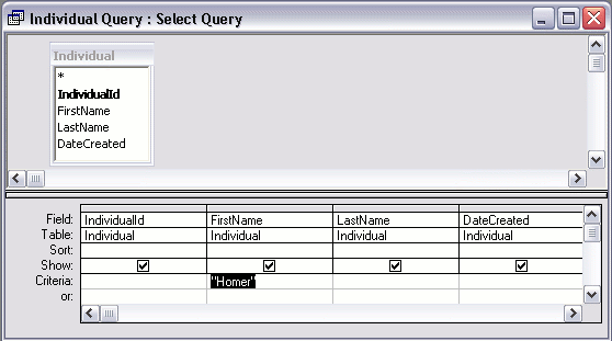
Database management systems usually offer a "design view" for your queries. Design view enables you to pick and choose which columns you want to display and what criteria you'd like to use to filter the data.
Here's an example of design view in Microsoft Access:
Database query - design view
When using design view, the database system actually uses SQL (behind the scenes) to generate the query.

Adding Data to a Database


There are a number of ways you can enter data into a database table. The method you choose will largely depend on your context.
You will need to choose from the following methods:
  • Direct entry
  • Form
  • Structured Query Language (SQL)
  • Website or other application
Here's an explanation of those methods.

Direct entry

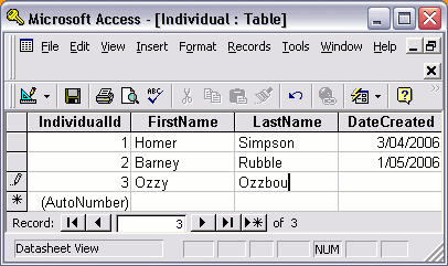
You can type directly into the table while it's in Data Sheet view. Initially, this may seem like the quickest and easiest method, but it's not suitable if you have lots of data, and/or if non-technical users need to enter data.
Adding data using the direct entry method

Form

Adding data using a form
If you use a desktop database program (such as MS Access), you can set up a form, so that non-technical users can enter data into the form. Once they submit the form, the data is automatically inserted into our table. The form could insert data into multiple tables too - saving you from having to open up each table to manually insert the data.
Most enterprise database systems don't have the ability for setting up a form. This is probably because they're designed for larger scale applications with hundreds, thousands, or even millions of users. In this environment, a form would be created through other means (for example, using HTML).
Applications such as Access provide a form wizard, which steps you through the process to building a form.

Structured Query Language (SQL)

SQL view
You can use a programming language called SQL to insert the data (we could also have used SQL to create the database and tables if we'd wanted to). One advantage of this is that you can save your SQL script for re-use. This could be handy if you need to insert the data into multiple databases.
It's also useful to create scripts that insert "lookup" data - this is generally a base set of data that never changes (such as Countries, Cities, etc). If you ever need to rebuild your database, you can simply run your ready made script against it (which saves you from manually re-entering the data).

Website or other application

You could build a program that uses the database to store and retrieve data. The person entering the data doesn't need to have direct access to the database. They don't even need to have database software. By using SQL, your database could be part of a larger application - such as a website.
This is probably the most common method of adding data to a database. If you've ever registered with a website, your details would have been inserted into a database using this method.

Creating Database Tables


With database management systems, you need to create your tables before you can enter data. Just as you can create a database programatically, you can create your tables programatically too.

Option 1: Programatically

The following is an example of creating a new table. Note that we are specifying the name of the table, the name of each column, and the data type of each column. More parameters can be added to this example if your requirements are more specific.
Code

Option 2: User Interface

Database management systems usually have a "Design View" for creating tables. Design view enables you to create the names of each column, specify the type of data that can go into each column, as well as specifying any other restrictions you'd like to enforce. Restricting the data type for each column is very important and helps maintain data integrity. For example, it can prevent us from accidentally entering an email address into a field for storing the current date.
More parameters can be added against each column if you require them. For example, you could specify a default value to be used (in case the field has been left blank by the user).
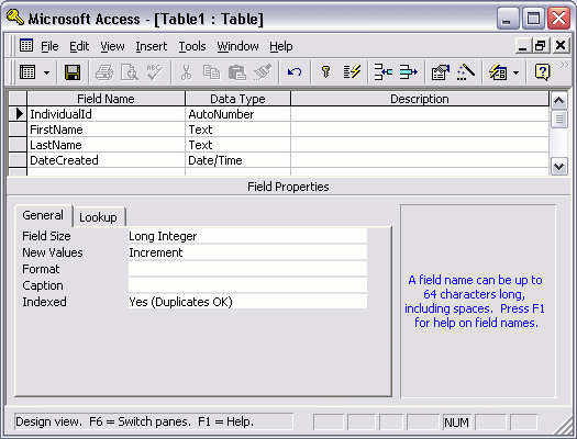
When you create a table via the user interface (or design view), depending on which database system you use, you should see something like this:
Database table - design view
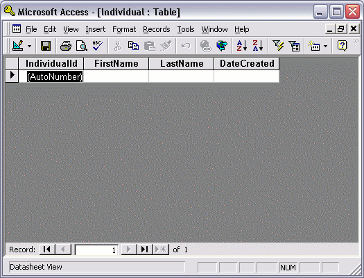
Once you've created your table in "design view", you can switch to "datasheet view" to see the resulting table. You should see something like this:
Database table in datasheet view
OK, so this is a blank table - it doesn't have any data yet. What we have is a table that contains the columns required before we can enter any data.
So, now that we have a blank table, let's look at how to add data.